Measuring a Magnetic Dipole via Harmonic Oscillation

Introduction

Oscillations are among the most important motions to understand when dealing with physics on both a macro and micro scale; the oscillation of an object can be used to determine specific properties of said object, especially in the case of magnets and magnetic fields¹. In this case, we placed a cue ball containing a magnetic dipole in a constant magnetic field generated by an approximately² Helmholtz coil (so as to create a consistent magnetic field in the area that the cue ball was placed) and allowed it to oscillate. By changing the current through the coil³ and measuring the change in the frequency of oscillations, we were able to calculate the strength of the magnetic dipole. Given the input of the current (our independent variable) and the output of the frequency (our dependent variable), a simple way to draw a comparison between the two was to find a method by which we could linearize the graph of the values such that the slope of the line would be our value for the magnetic dipole. To linearize this graph, we could not have just placed the raw values on the axes, rather we needed to calculate values that depended on these raw values.

Newton’s second law states that the sum of the torques on a system will be equal to the moment of inertia times the angular acceleration, which is written as

\[\tau=I\alpha,\tag1\]

where $I$ is the moment of inertia and $\alpha$ is angular acceleration; angular acceleration is defined as the second derivative of angular position, such that

\[\alpha=\frac{d^2\theta}{dt^2},\tag2\]

where $\theta$ is the angular position and $\alpha$ is the angular acceleration. The equation for the magnetic torque can be written as

\[\tau=-\mu B\sin(\theta),\tag3\]

where $\tau$ is the torque, $\mu$ is the magnetic dipole moment, and $B$ is the magnitude of the magnetic field. We then assumed a small angle for the magnetic torque, allowing us to simplify that equation to just

\[\tau=-\mu B\theta,\tag4\]

wherein we could then find an equation for $\theta$, based on the system being a harmonic oscillator, to be

\[\theta=\cos(\omega t),\tag5\]

where $\omega$ is the frequency of oscillation. With these substitutions we found a slightly simpler equation than we would have gotten without the small angle approximation, that being

\[-\mu B\cos(\omega t)=I\frac{d^2}{dt^2}\cos(\omega t).\tag6\]

From there we simplified along the following steps:

\[\begin{align} -\mu B\cos(\omega t)&=I(-\omega^2\cos(\omega t)),\tag{7a}\\ -\mu B&=-\omega^2I,\tag{7b}\\ \mu B&=\omega^2I,\tag{7c} \end{align}\]

While our goal was to find $\mu$, we did not simply solve this equation for $\mu$, we wanted to create an equation for some function to which we would be able to fit our data (including any uncertainty bars). We found that the simplest route by which this could be done would be to create an equation for a line, i.e. $y=mx+b$, wherein the slope we found was to be $\mu$. With this in mind, we rearranged the equation to find

\[\omega^2=\mu\frac BI.\tag8\]

Experimental Methods

The primary apparatus used for this experiment was the TeachSpin M$\tau$1-A,⁴ which comprises of the aforementioned near Helmholtz coils, an air pump, and a power supply. The oscillator was built out of a cue ball, with a magnetic dipole at the center. Once the cue ball was placed in the center, it was pushed upwards by the air pump, this would remove nearly all the friction that would otherwise have been caused by the cup holding the ball. When the current from the power supply was applied to the coils, a magnetic field was generated. The cue ball was displaced by some small angle from equilibrium and released. To find the frequency of the resulting oscillation, all three members of our lab group measured the time with their own stop watch over ten oscillations, and these times were then averaged so as to attain the most accurate measurement of time.

Results

To begin with any of the calculations for this lab, we needed to find the moment of inertia of the cue ball. As the ball is a sphere, we used the equation for the moment of inertia of a sphere:

\[I=\frac 25mr^2,\tag9\]

where $m$ is the mass and $r$ is the radius of the cue ball. We measured $m=137.65g\pm0.01g$ and $r=2.68cm\pm0.005cm$, resulting in $I=395.4629g\cdot cm^2\pm0.0037g\cdot cm^2$. We also need some means by which to calculate our $B$, for this we used an equation derived from the Biot-Savart Law for Helmholtz Coils:

\[B=\left(\frac 45\right)^{3/2}\frac{\mu_0Ni}{R},\tag{10}\]

where $x$ is the distance between the coils. Given the measurements taken for our system, this simplifies to $B=1.36\cdot i \cdot mT/A$.

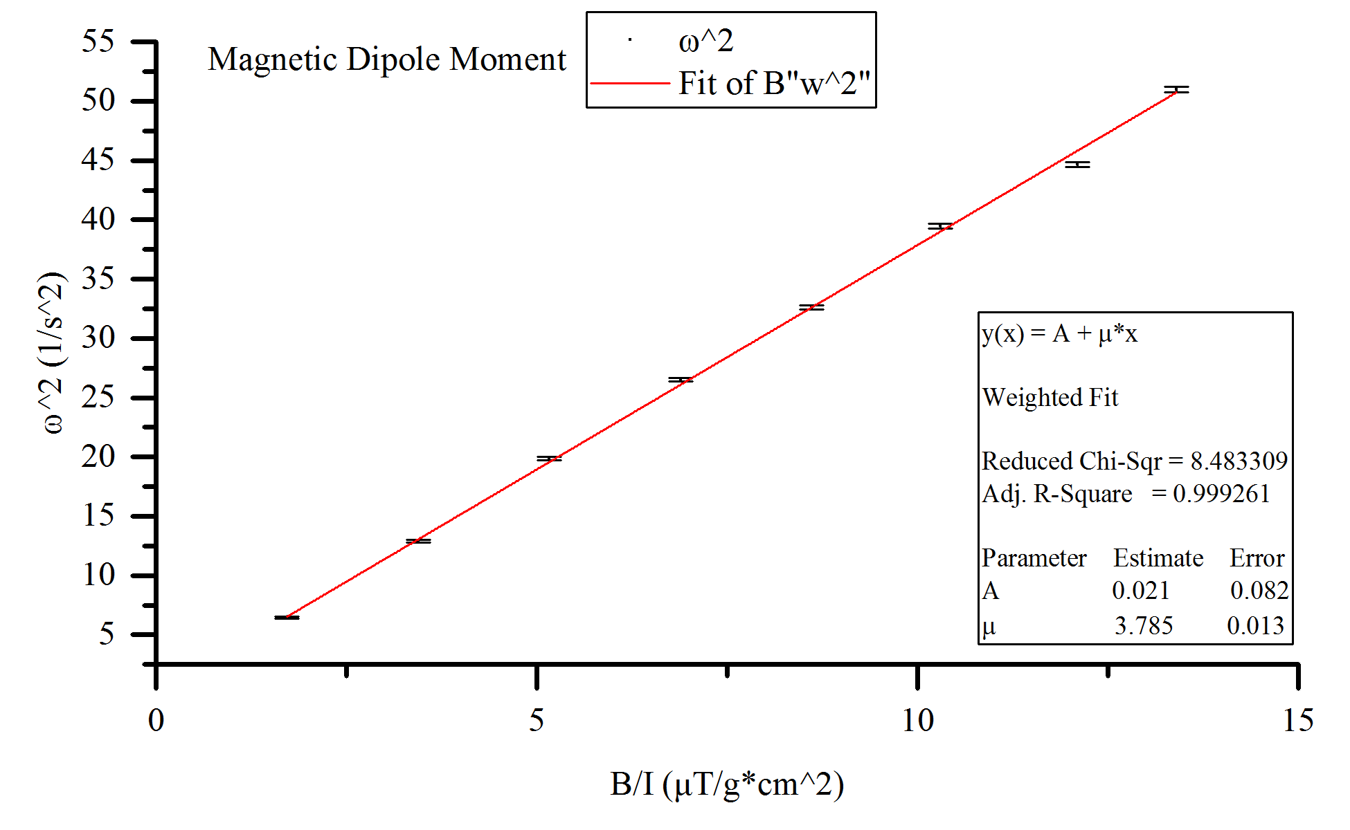
FIGURE 1. Graph of all collected data with a weighted fit to a straight line, the slope of which is our desired value for $\mu$. The uncertainty on each point was propagated from the standard error in the measured time, as determined by the standard deviation of three collected samples.

To create a graph from which $\mu$ can be found, we needed to create a linear fit such that $\mu$ would be the slope. This was achieved by graphing $\omega^2$ versus $B⁄I$ as seen in Figure 1.

The curve fit found an intercept of the line at $0.02118\pm0.2406$ making it statistically consistent with zero, and slope of $\mu=0.3785\pm0.0013 A\cdot m^2$ (the slope given by the fit was $3.785$, but the units of the x-axis were in microteslas per gram centimeter squared when the desired units were teslas per gram meter squared, a factor of ten greater and therefore the slope should be one tenth of that reported by this fit).

Discussion

This method of measuring the moment of an object by timing its oscillations in a field of applied forces is possibly the most efficient method as oscillations are directly affected by the moment. As such, it is not the methodology of this experiment that would need to be changed to more accurately measure the moment. The first adjustment to be made that could help produce more accurate results would be to use a proper Helmholtz coil, this would simplify the math needed and therefore result in there being less possible errors. Measuring the time of the oscillations for a greater amount of oscillations could also help to remove errors in the measurements that would result in less errors in the results as well.

Acknowledgements

T.H. would like to thank R. Scott and L. Syverson for help with data collection.

References